Having your data spread out across different spreadsheets is a common challenge. You might have sales figures in one file, inventory data in another, and customer information in a third sheet. When you need to pull that information together to build a dashboard or a summary report, the default solution is often manual copying and pasting.

What if your Google Sheets could talk to each other, automatically updating your reports whenever the source data changes?

In this guide, we’ll explore all the powerful ways to import data between different Google Sheets.

Also see: Create Stock Dashboard in Google Sheets

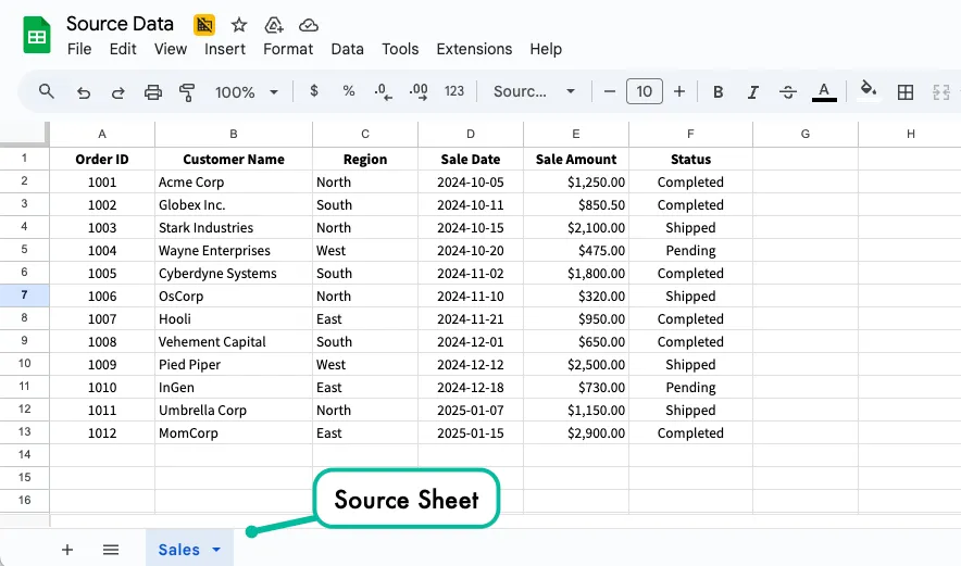
For our examples, we’ll use a source Google Spreadsheet with a sheet named Sales. This sheet contains customer names, regions, sales amounts, and other details that we’ll be importing into other Google Sheets.

Import Data with IMPORTRANGE

The IMPORTRANGE function in Google Sheets allows you to bring in data from an entirely different spreadsheet, maintaining a live connection between the source and destination. This live link ensures that your reports and dashboards always reflect the most up-to-date information, without needing to manually copy or update data.

The only requirement for IMPORTRANGE is that the source spreadsheet must be accessible to the person importing the data. If you’re importing from a sheet you don’t own, ensure the owner has granted you editor or viewer access.

To use the IMPORTRANGE function, you need to provide the URL of the source spreadsheet and the range of cells you want to import. For example, if you want to import the data from the Sales sheet, the range would be something like Sales!A1:F50. If the sheet name contains spaces, you need to wrap it in single quotes like 'Q3 Sales'!A1:F50.

The syntax for the IMPORTRANGE function is simple:

=IMPORTRANGE(spreadsheet_url, range_string)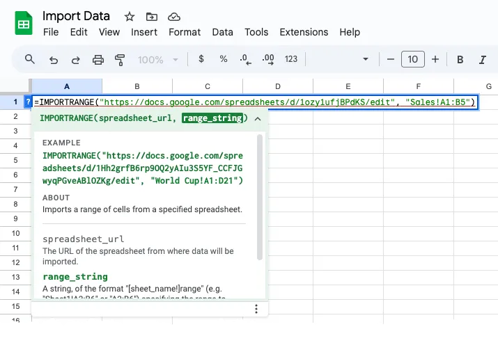

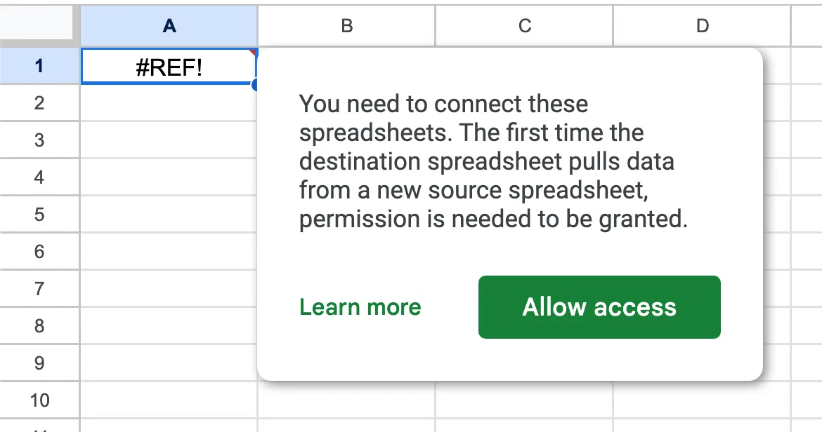
The first time you add this function to your spreadsheet cell, it will return a #REF! error. This simply means Google Sheets needs your permission to access the source spreadsheet. Hover your mouse over the error and click on Allow access to grant access. This authorization is remembered, so you only need to do it once per destination spreadsheet.

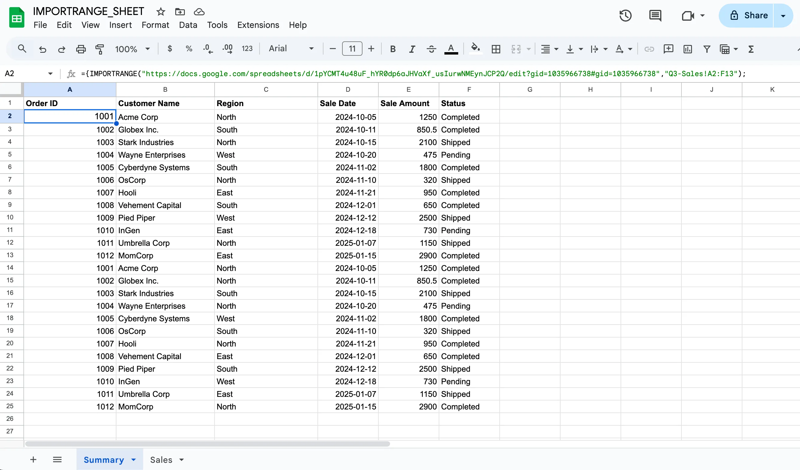
Going back to our previous example, if we wish to import the header row and the first 12 rows of data from the Sales sheet into a new sheet, our formula would look like this:

=IMPORTRANGE("https://docs.google.com/spreadsheets/d/1234567890/edit", "Sales!A1:F13")

Combine Multiple Ranges with IMPORTRANGE

The power of IMPORTRANGE isn’t limited to pulling a single range. You can combine data from multiple ranges -even from different sheets or spreadsheets - into one continuous list using array literals {}.

The array syntax {} tells Google Sheets to build a custom array, or list, of data based on your instructions. There are two primary ways to arrange your combined data:

Vertical Stacking (Place data one on top of the other)

This is the most common and powerful way to combine data. By separating your IMPORTRANGE formulas with a semicolon;, you can merge data from different sheets (or even different spreadsheets) into a single list where the data is placed one on top of the other.

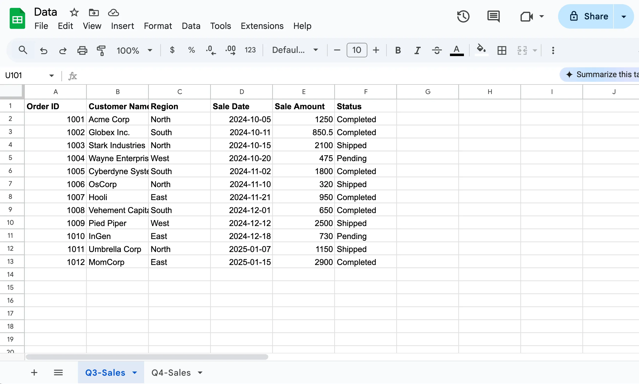
For example, if you have sales data split between “Q3-Sales” and “Q4-Sales” sheets in your source spreadsheet, you can combine them vertically using the formula:

={IMPORTRANGE(sheet_URL,"Q3-Sales!A2:F13"); IMPORTRANGE(sheet_URL,"Q4-Sales!A2:F13")}

This formula first pulls the specified range from “Q3-Sales.” The semicolon then tells it to append the data from “Q4-Sales” directly below the Q3 data.

🔥 Please note that the number of columns selected in each IMPORTRANGE formula are the same else Google Sheets will return an error saying In ARRAY_LITERAL, an Array Literal was missing values for one or more rows.

💡 We usually start from cell A2 in both ranges. This is a common practice to avoid importing the column headers twice, giving you a clean, continuous list of data.

Horizontal Stacking (Place data side-by-side)

This method is useful when you have data that is spread across multiple columns in different sheets. It allows you to combine data from different sheets into a wider table with more columns.

To place ranges next to each other horizontally, you use the same array syntax but separate the formulas with a comma inside the curly braces {}. Here you can have different number of rows in each range but the number of columns in each range of the IMPORTRANGE formula must be the same.

Let’s say you have the customer names in the Customer sheet and their address details in an Address sheet.

={IMPORTRANGE(sheet_URL,"Customer!A2:B6"), IMPORTRANGE(sheet_URL,"Address!A2:C6")}

The above formula pulls customer names from the first range and places the address details from the second range in the columns immediately to the right.

Note on Performance

You can absolutely use multiple IMPORTRANGE formulas in one Google Sheet. However, it’s important to remember that each formula creates a live connection to an external file. If you have dozens of these functions in a single sheet, it can slow down your calculations, as it constantly checks for updates in source sheets.

For optimal performance, use one IMPORTRANGE formula to bring the entire raw dataset into a new, dedicated tab in your report. Then, use multiple QUERY or FILTER formulas in your dashboard that reference this local, imported data.

This way you can only create one external connection, and all subsequent filtering is done inside your sheet, which is significantly faster.

Google Maps Formulas for Google Sheets

Conditional Imports with the QUERY function

While IMPORTRANGE is an easy option for importing data into your sheet, its true potential is unlocked when you control exactly what data comes through. Importing an entire dataset is often unnecessary; you typically only need specific rows – like inventory from a certain warehouse, or sales for a specific period.

This is where the QUERY function becomes your most powerful ally. By wrapping your IMPORTRANGE in a QUERY, you can move beyond simple importing and begin pulling data based on a specific condition(s). The syntax for the QUERY function is as follows:

=QUERY(IMPORTRANGE("spreadsheet_url", "range"), "Your Query Statement")

The spreadsheet_url is the URL of the spreadsheet from where data will be imported. The range tells Google Sheets exactly which sheet and which cells you want to import. The Query Statement is your filter (eg: where Col3 = ‘Confirmed’).

How to use QUERY function - Examples

Get All Data for a Specific Region

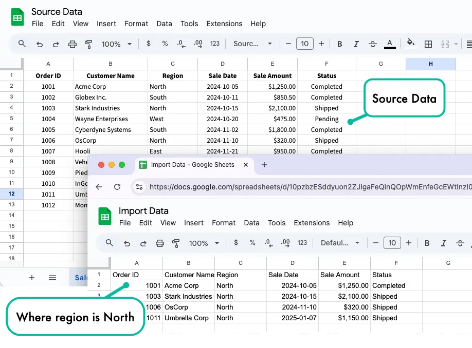
Our source Google Spreadsheet has a sheet named Sales that contains the customer name, the region, sale amount and other details that we would like to import into our destination sheet. The IMPORTRANGE function will help but we only want to import the data for the North region.

=QUERY(IMPORTRANGE("URL", "Sales!A1:F13"), "SELECT * WHERE Col3 = 'North'")

• SELECT * means that we want to import all columns from the source sheet.
• WHERE Col3 = ‘North’ is the filter. It tells the query to only return rows where the third column (Col3, which is Region) is equal to North. Note that the text values are case-sensitive and must be in single quotes.

The QUERY function does not see the original spreadsheet but the final data array that is returned by the IMPORTRANGE function. Therefore, it refers to the columns of the resulting array by their order: Col1 is the first column of your imported range, Col2 is the second, and so on.

Combine Multiple Conditions (AND)

You need a report of all “Completed” sales in the “South” region. The AND keyword lets you chain multiple conditions. The query will only return rows that satisfy both the conditions:

=QUERY(IMPORTRANGE("URL", "Sales!A1:F13"), "SELECT * WHERE Col3 = 'South' AND Col6 = 'Completed'")

Filter by a List of Possible Values (OR)

You want to see all sales data from either the “East” or “West” regions combined in one list. The OR keyword returns rows that match either condition, allowing you to check for multiple possible values in the same column.

=QUERY(IMPORTRANGE("URL", "Sales!A1:F13"), "SELECT * WHERE Col3 = 'East' OR Col3 = 'West'")

Filter by a Numerical Value

You need to generate a list of all high-value sales where the sale amount is over $1,000. You can use standard comparison operators >, <, >=, <=, = for numbers. Notice that numbers and currency values are not placed in quotes.

=QUERY(IMPORTRANGE("URL", "Sales!A1:F13"), "SELECT * WHERE Col5 > 1000")

Select Specific Columns with Sorting

You want a clean report showing just the Customer Name and Sale Amount for high-value sales, with the largest sales appearing first.

=QUERY(IMPORTRANGE("URL", "Sale!A1:F12"), "SELECT Col2, Col5 WHERE Col5 > 1000 ORDER BY Col5 DESC")

• SELECT Col2, Col5 specifies that we only want to import the “Customer Name” and “Sale Amount” columns.
• ORDER BY Col5 DESC sorts the results based on the “Sale Amount” column (Col5) in descending order. Use ASC for ascending order.

Filter by a Date Range

You need to see all sales that occurred in the fourth quarter of 2024 (from October 1st to December 31st). When working with dates in QUERY, you must use the date keyword followed by the date in ‘YYYY-MM-DD’ format, enclosed in single quotes.

=QUERY(IMPORTRANGE("URL", "Sales!A1:F13"), "SELECT * WHERE Col4 >= date '2024-10-01' AND Col4 <= date '2024-12-31'")

Find Partial Text Matches

You want to find all sales made to any company with “Inc” in its name. The contains operator is perfect for finding a substring within a text field.

=QUERY(IMPORTRANGE("URL", "Sales!A1:F12"), "SELECT * WHERE Col2 contains 'Inc'")

You can also use starts with, ends with or matches operators to filter text values based on regular expressions.

Limiting the Number of Results

You want to create a Top 5 leaderboard showing the largest sales. The LIMIT clause allows you to restrict the number of rows returned.

=QUERY(IMPORTRANGE("URL", "Sales!A1:F12"), "SELECT * ORDER by Col5 DESC LIMIT 5")

Aggregating Data to Create Summaries

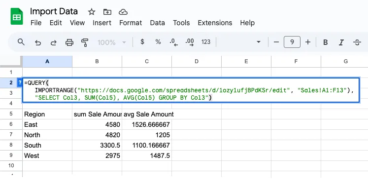
Instead of a long list of sales, you want a summary table showing the total sales value for each region. The GROUP BY clause aggregates rows and lets you perform calculations on them with functions like SUM(), COUNT(), and AVG().

=QUERY(IMPORTRANGE("URL", "Sales!A1:F12"), "SELECT Col3, SUM(Col5), AVG(Col5) GROUP BY Col3")

The GROUP BY Col3 clause scans the Region column and finds all the unique values (North, South, East, West). It then creates a single output row for each region. The aggregate functions SUM(Col5) and AVG(Col5) then calculate the total and average sales amount for all rows that belong to that region.

Other useful aggregate functions include COUNT(), MAX(), and MIN().

Rename Column Titles in QUERY output

Google Sheets automatically names the columns in the output of a QUERY function based on the formula used. For example, if you use SELECT Col3, SUM(Col5) GROUP BY Col3, the output will have column titles like sum Sale Amount that are not very descriptive. The LABEL clause lets you rename these output headers for better readability.

=QUERY(IMPORTRANGE("URL", "Sales!A1:F12"), "SELECT Col3, SUM(Col5) GROUP BY Col3 LABEL SUM(Col5) 'Total Sales', Col3 'Sales Region'")

The syntax is LABEL column_to_rename new_column_name. You can chain multiple labels with a comma. This only changes your header in your output, it does not affect the original source data in any way.

Formatting Date and Numbers

You can control how numbers and dates are displayed directly within your query output using the FORMAT clause. This is great for applying currency symbols or standardizing date formats without manually formatting the entire column.

=QUERY(IMPORTRANGE("URL", "Sales!A1:F12"), "SELECT Col3, SUM(Col5) GROUP BY Col3 LABEL SUM(Col5) 'Total Sales' FORMAT SUM(Col5) '$\#,\#\#0.00'")

The pattern '$\#,\#\#0.00' tells Sheets to display the number with a dollar sign, a comma for the thousands separator, and two decimal places. This is purely visual, the underlying value is still a number. You could format a date with a pattern like mmm d, yyyy to get Jul 15, 2025.

Transpose Data with PIVOT

You can use the PIVOT clause in your QUERY function to transform your data from a list into a wide, cross-tabulated summary, similar to a traditional Pivot Table. This is particularly useful when you want to see how values in one column (like sales amounts) are distributed across categories from another column (like regions).

=QUERY(IMPORTRANGE("URL", "Sales!A1:F12"), "SELECT Col3, SUM(Col5) GROUP BY Col3 PIVOT Col6")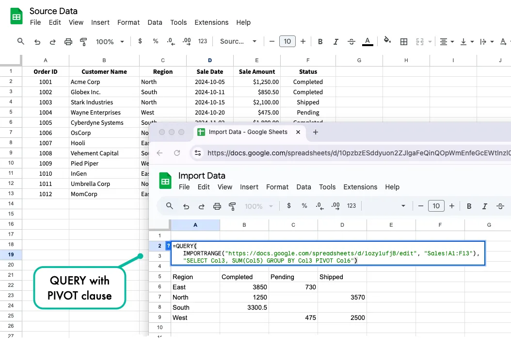

This query does three things:

• GROUP BY Col3 creates a unique row for each region.
• SUM(Col5) decides what value will be calculated for the cells.
• PIVOT Col6 takes the unique values from the “Status” column (Completed, Shipped, Pending) and turns them into their own columns. The results is a table showing the total sales value for each region, broken down by status.

Using a Cell Reference as a Condition

You can make your queries dynamic and interactive by building the query string to reference another cell. This is the foundation for creating dashboards that react to user input.

To filter by text from a cell (e.g., cell G1 contains the region name), use this formula:

=QUERY(IMPORTRANGE("URL", "Sales!A1:F12"), "SELECT * WHERE Col3 = '"&G1&"'")

Notice how we use the ampersand & operator to concatenate the value from cell G1 into the query string. Text values need to be enclosed in single quotes within the QUERY string.

If you were filtering by a number from cell G1, the syntax would be simpler:

=QUERY(IMPORTRANGE("URL", "Sales!A1:F12"), "SELECT * WHERE Col5 > " & G1)

Use QUERY with Multiple Ranges

While the QUERY function only takes a single data range as its input, you can use the curly braces {} syntax to create a single combined range from multiple sheets and then apply the QUERY function to filter that combined data. Here is an example:

=QUERY(
   {
      IMPORTRANGE("URL", "Q3-Sales!A1:F12"),
      IMPORTRANGE("URL", "Q4-Sales!A1:F12")
   },
   "SELECT * WHERE Col6 = 'North'"
)

Here’s how this formula works step by step:

• Google Sheets evaluates the expressions inside the curly braces first. This means it executes both IMPORTRANGE functions and combines their results into a single unified table.
• The semicolon between the IMPORTRANGE functions tells Sheets to stack the results vertically - the second range will appear directly below the first range.
• Once the data is combined into a single vertical table, the QUERY function processes this merged dataset as if it were a single table.

Important: When stacking ranges this way, each IMPORTRANGE must return the same number of columns.

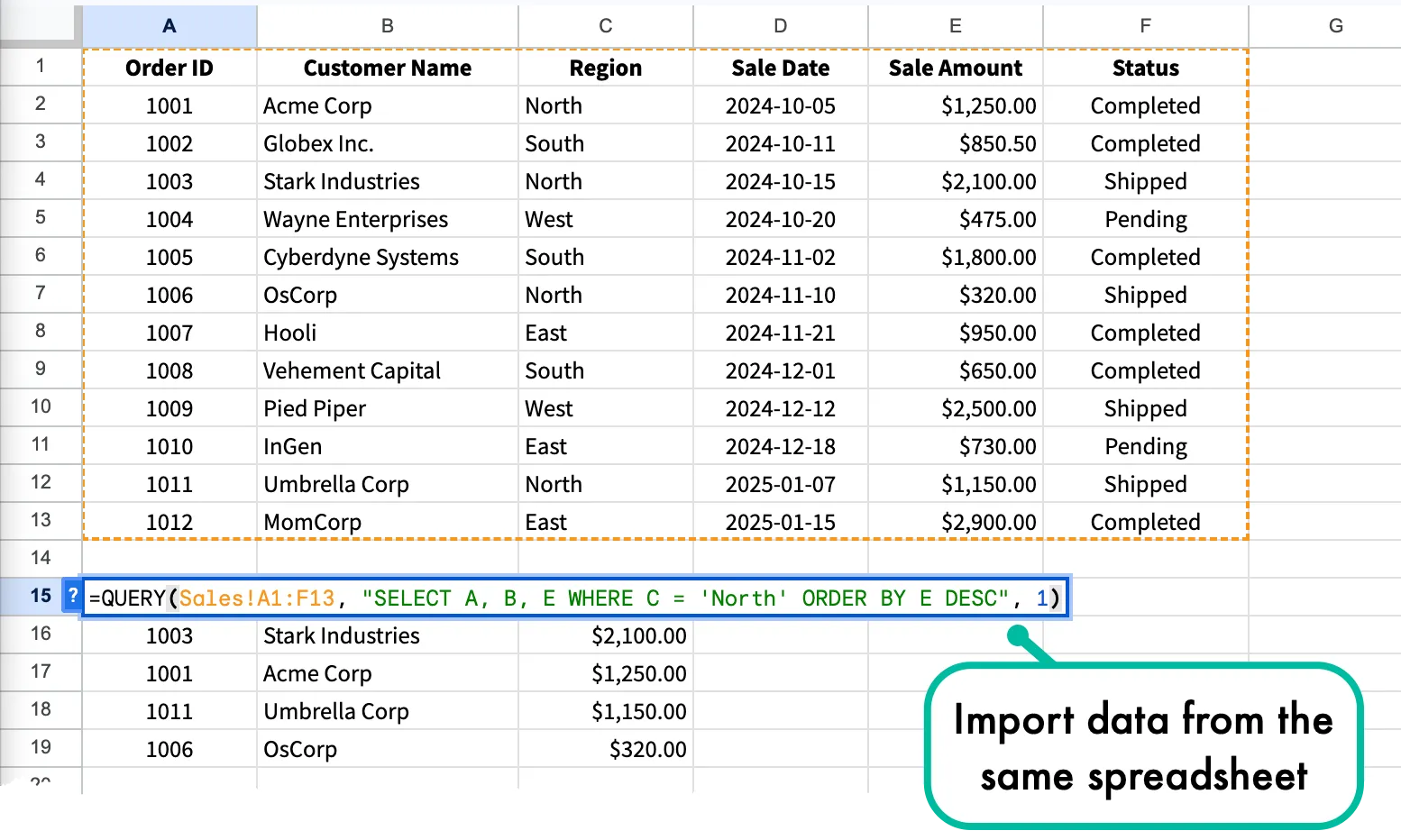
Import Data from the Same Spreadsheet

While IMPORTRANGE is essential for pulling data from separate files, what if your data resides in a different tab within the same spreadsheet? For this scenario, you don’t need the IMPORTRANGE function but directly reference the cell in the source sheet.

To reference a single cell from another sheet, you simply type =, followed by the sheet name, an exclamation mark, and the cell you want to pull the data from.

=Sales!E14

To reference a range of cells from another tab, you use the same syntax as above but wrap it in curly braces {}. This instructs Google Sheet to output the entire array of data, not just a single value.

={Sales!A1:D10}

A common pattern is to combine local cell referencing with the QUERY function. This allows you to keep your raw data in one tab while creating multiple, filtered reports in other tabs – all within a single, fast loading spreadsheet.

When you use QUERY on a range from within the spreadsheet, you can directly use the actual column letters (A,B,C) in your QUERY statement, instead of using the column numbers (Col1, Col2, Col3). This is because QUERY is referencing the local sheet directly and can see its structure.

=QUERY(Sales!A1:F12, "SELECT A, B, E WHERE C = 'North' ORDER BY E DESC")

The above QUERY function pulls the data from the Sales sheet and filters it to only include the rows where the Region column is equal to North. It then sorts the results by the Sale Amount column in descending order.

Importing Data - Which Method to Use?

Whether your data lives in another spreadsheet or in another tab of the same sheet, Google Sheets provides reliable and automated ways to import data and also ensuring that your reports and dashboards are always up to date.

To summarize:

• If you need to pull data from a completely different spreadsheet, your starting point will always be the IMPORTRANGE function.
• If you need to filter, sort or manipulate data, you should wrap your IMPORTRANGE inside a QUERY function.

Also see: Create Google Sheets Screenshots