Microsoft Excel provides a handy feature called “Quick Styles” to help you quickly format a selected range as a striped table. The table can have zebra lines meaning alternating rows are formatted with different colors.

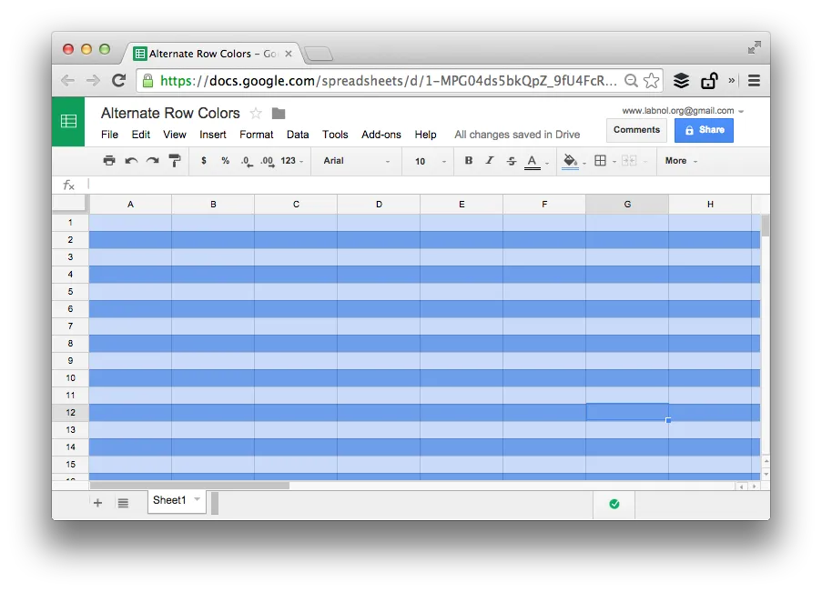
In Google Sheets, you can use conditional formatting combined with a simple Google Formula to create a table formatting like zebra strips. You can apply alternating colors to both rows and columns in Google Sheets easily.

Here’s the trick.

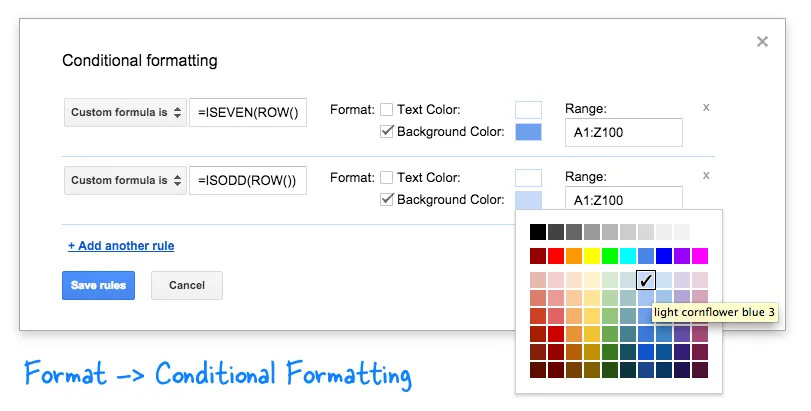
Open a Google Sheet and choose Conditional formatting from the Format menu. Select Custom Formula from the dropdown and put this formula in the input box.

=ISEVEN(ROW())

Select a Background color for the rule and set the range in A1 notation. For instance, if you wish to apply alternating colors to rows 1 to 100 for columns A to Z, set the range as A1

Click the “Add another rule” link and repeat the steps but set =ISODD(ROW()) as the custom formula and choose a different background color. Save the rules and the zebra stripes would be automatically applied to the specified range of cells.

Tip: If you wish to extend this technique to format columns with different colors, use the =ISEVEN(COLUMN()) formula. Simple!