How to Use Conditional Formatting in Google Sheets to Highlight Information
Conditional formatting in Google Sheets allows you to apply automatic formatting to cells in spreadsheets that meet certain criteria. Check out some practical examples and master conditional formatting in Google Sheets.
Conditional formatting in Google Sheets makes it easy for you to highlight specific cells that meet a specific criteria. For instance, you can change the background color of a cell to yellow if the cell value is less than a certain number. Or you can choose to highlight an entire row or column if certain conditions are met.
Highlight Individual Cells
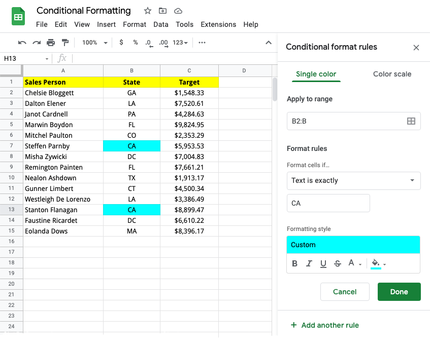
For this example, we have a sales chart that lists the names of salespeople, their state and the total sales target. We would like to highlight individual cells in the State column if the salesperson is from California.
Go to the Format menu, choose Conditional Formatting, and click Add Condition. Here, choose the range as B2:B and the format condition as Text is Exactly. Then, enter the text CA in the text box, choose a custom background color and click Done.
Highlight Entire Row
For the same Sales chart, we would now like to highlight entire rows where the sales target is more than $8,000.
Inside the formatting rule, set the range as A2:C since we would like to apply formatting to the entire table. Next, choose Custom Formula is for the formatting rules condition and set the criteria as =$C2>8000.
If you would like to highlight rows where the sales target is within a range, say between $5000 and $7000, you can add the =ISBETWEEN($C2, 5000,7000) formula in the criteria box.
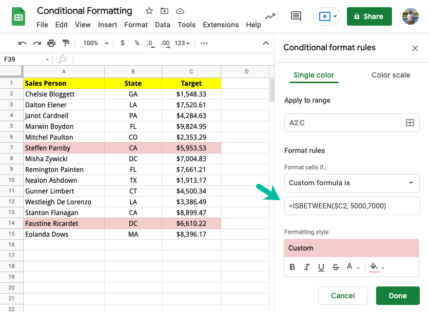
The $ in $C2 applies the formula to the entire column C while the missing $ in front of the number 2 allows it to increment.
If you want to highlight rows where the sales target is more than the average sales target, you can either use =IF(AVERAGE($C2:C)<$C2,1) or =$C2>average($C2:C) formula in the criteria box.
If you wish to highlight a row that contains the maximum value for sales, you can use the =MAX() formula in the criteria box.
=$C:$C=max($C:$C)Also see: Highlight Duplicate Rows in Google Sheets
Formatting based on two cells
In the same Sales table, we would like to highlight salespersons who are responsible for a specific state (say, “CA”) and who have a sales target of more than $5,000.
We can achieve this by applying multiple conditions using the AND function as shown below:
=AND(C2>5000, B2="CA")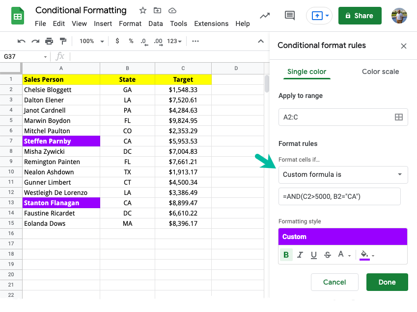
Conditional Formatting base on Date
Our table has a list of invoice and the date when the invoice is due. We’ll use conditional formatting to highlight invoices that are past due for more than 30 days and send them email reminders.
=DAYS(TODAY(),$B:$B)>=30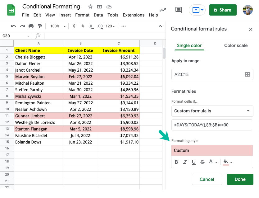
In another example, we have a list of students and their date of birth. We can use Date functions like to highlight students who are older than 16 years old and whose date of birth is in the current month.
=AND(YEAR(TODAY())-YEAR($B2)>=16,MONTH($B2)=MONTH(TODAY()))Heatmaps - Format Cells by Color Scale
Our next workbook contains a list of US cities and their average temperatures for various months. We can use Color Scales to easily understand the temperature trends across cities. The higher values of the temperature are more red in color and the lower values are more green in color.
Mark Rows Containing one of the values
With conditional formatting in Google Sheets, you can easily highlight rows that contain a specific value. For example, you can highlight all rows that contain the value CA in the State column.
However, if you want to highlight rows that contain one of multiple values, you can either use the OR function or, better still, use Regular Expressions with the custom formula.
This formula will highlight all rows that contain either CA or NY or FL in the State column.
=REGEXMATCH(UPPER($B:$B), "^(CA|NY|FL)$")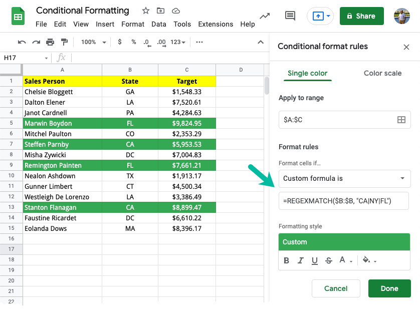
Alternatively, you may have a list of states listed in another sheet and use MATCH with INDIRECT to highlight rows that contain one of the states.
=MATCH($B1, INDIRECT("'List of States'!A1:A"),0)Apply Conditional Formatting to Entire Column
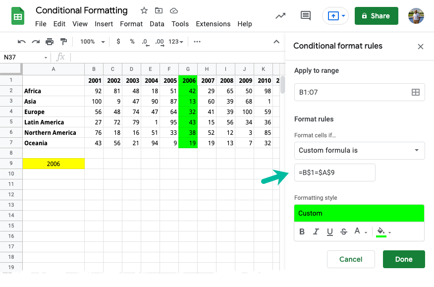
Until now, we have explored examples of highlighting individual cells or entire rows when certain conditions are satisfied. However, you can use conditional formatting to highlight entire columns of a Google Sheet.
In this example, we have sales for different years per geographic region. When the user enters the year in cell A9, the corresponding column is highlighted in the sales table. The custom formula will be =B$1=$A$9. Notice that the $ is used with the number in the cell reference since the check is made only in the first row.
Conditional Formatting with Google Apps Script
If you were to apply the same conditional rules to multiple Google Spreadsheets in one go, it is recommended that you automate Google Apps Script else it will take more time to apply the formatting manually.
const applyConditionalFormatting = () => {
  const sheet = SpreadsheetApp.getActiveSheet();

  const color = SpreadsheetApp.newColor().setThemeColor(SpreadsheetApp.ThemeColorType.BACKGROUND).build();

  const rule1 = SpreadsheetApp.newConditionalFormatRule()
    .setRanges([sheet.getRange('B:B')])
    .whenTextEqualTo('CA')
    .setUnderline(true)
    .setBold(true)
    .setBackground(color)
    .build();

  const rule2 = SpreadsheetApp.newConditionalFormatRule()
    .setRanges([sheet.getRange('A1:C15')])
    .whenFormulaSatisfied('=$C1>5000')
    .setBackground('green')
    .setFontColor('#00FF00')
    .build();

  const conditionalFormatRules = sheet.getConditionalFormatRules();
  conditionalFormatRules.push(rule1);
  conditionalFormatRules.push(rule2);

  sheet.setConditionalFormatRules(conditionalFormatRules);
};
Please check the documentation of ConditionalFormatRuleBuilder for more details. This will also help you copy conditional formatting rules from one spreadsheet to another.

Amit Agarwal
Google Developer Expert, Google Cloud Champion
Amit Agarwal is a Google Developer Expert in Google Workspace and Google Apps Script. He holds an engineering degree in Computer Science (I.I.T.) and is the first professional blogger in India.
Amit has developed several popular Google add-ons including Mail Merge for Gmail and Document Studio. Read more on Lifehacker and YourStory